The Dataset
A term deposit is a cash investment held at a financial institution. Your money is invested for an agreed rate of interest over a fixed amount of time, or term. The bank has various outreach plans to sell term deposits to their customers such as email marketing, advertisements, telephonic marketing, and digital marketing.
Telephonic marketing campaigns still remain one of the most effective way to reach out to people. However, they require huge investment as large call centers are hired to actually execute these campaigns. Hence, it is crucial to identify the customers most likely to convert beforehand so that they can be specifically targeted via call.
The data is related to direct marketing campaigns (phone calls) of a Portuguese banking institution. The classification goal is to predict if the client will subscribe to a term deposit (variable y).
Check Python version. This be useful when creating a production environment
!python -V
import numpy as np
import pandas as pd
import matplotlib.pyplot as plt
import seaborn as sns

import sklearn
sklearn.__version__ # note sklearn version too
train_df = pd.read_csv("train.csv", sep=";")
test_df = pd.read_csv("test.csv", sep=";")
print(train_df.shape)
print(test_df.shape)
test_df.head()
train_df.info()
test_df.info()
DictVectorizer
Encode the categorical columns using DictVectorizer.
from sklearn.feature_extraction import DictVectorizer

dv = DictVectorizer()

trainX = train_df.drop(columns=["y"])
trainy = train_df["y"]

testX = test_df.drop(columns=["y"])
testy = test_df["y"]

trainy = trainy.replace({"no":0, "yes": 1})
testy = testy.replace({"no":0, "yes": 1})
trainX = dv.fit_transform(trainX.to_dict(orient="records")).toarray()

testX = dv.fit_transform(testX.to_dict(orient="records")).toarray()
train_df.columns.sort_values()
print(dv.get_feature_names_out())
Unlike other encoders, DictVectorizer are more flexible and are very easy to apply to new data.
How it works
- Convert the dataframe to a dictionary using
.to_dict(orient="records") - Transform the dict dataframe using
dv.fit_transform(), where dv is the DictVecortizer object. - Convert to array to avoid errors during model training:
to_array.
This encodes columns in the dataframe that are categorical, and retain values of columns that are non-categorical.
The two cells above shows a comparison of the columns in the dataframe vs the columns in the dictvectorizer. You may agree that it looks similar to one-hot-encoding, concatenated to non-catgeorical columns.
Train the Model
!pip install xgboost
from xgboost import XGBClassifier

xgb = XGBClassifier()
xgb.fit(trainX, trainy)
y_pred = xgb.predict(testX)
from sklearn.metrics import classification_report, f1_score

print(classification_report(y_pred, testy))
print(f1_score(y_pred, testy))
While more feature engineering is encourged to increase the model's performance on class 1, we'll proceed to refactoring the codes and including experiment tracking with MLflow.
1. Put all used libraries into one cell.
# !pip install xgboost
!pip install mlflow --quiet;
import pandas as pd
from sklearn.feature_extraction import DictVectorizer
from sklearn.metrics import f1_score

from xgboost import XGBClassifier

import pickle # to export and load the model

import mlflow
If this is your first time with mlflow, it is one of those tools used in machine learning operations that helps to keep track of data, models, experiment results, etc. This helps you to know what models performed best, their hyperparameters, the time they took to run and names of the data used for the training. You can also choose to take track of the name of the data scientist that trained the model.
To start, one key thing to define is the experiment name.
# define experiment name. Give it any good name
mlflow.set_experiment("term-deposit-exp")
This creates a folder in your working directory, called "mlruns"/1 : where 1 represents the experiement serial number. If we create a new experiment it will be number 2
To see this, in your terminal,
- Create a virtual enviroment and install mlflow.
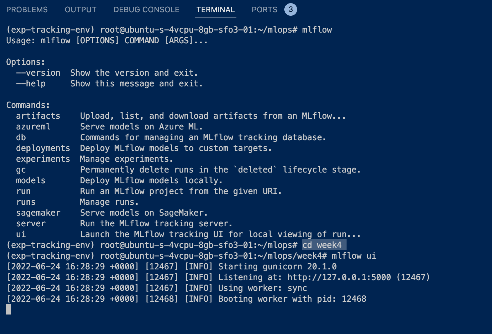
Remember to make your environment run on python 3.9 cdto this working directory where this particular notebook is located at. In my case, it isweek4. Then run the following:mlflow ui, as shown in the image below.

The Commands are actions we can carry out in mlflow. For a quick demo, mlflow ui will be used, but afterwards, we'll be working with mlflow server.
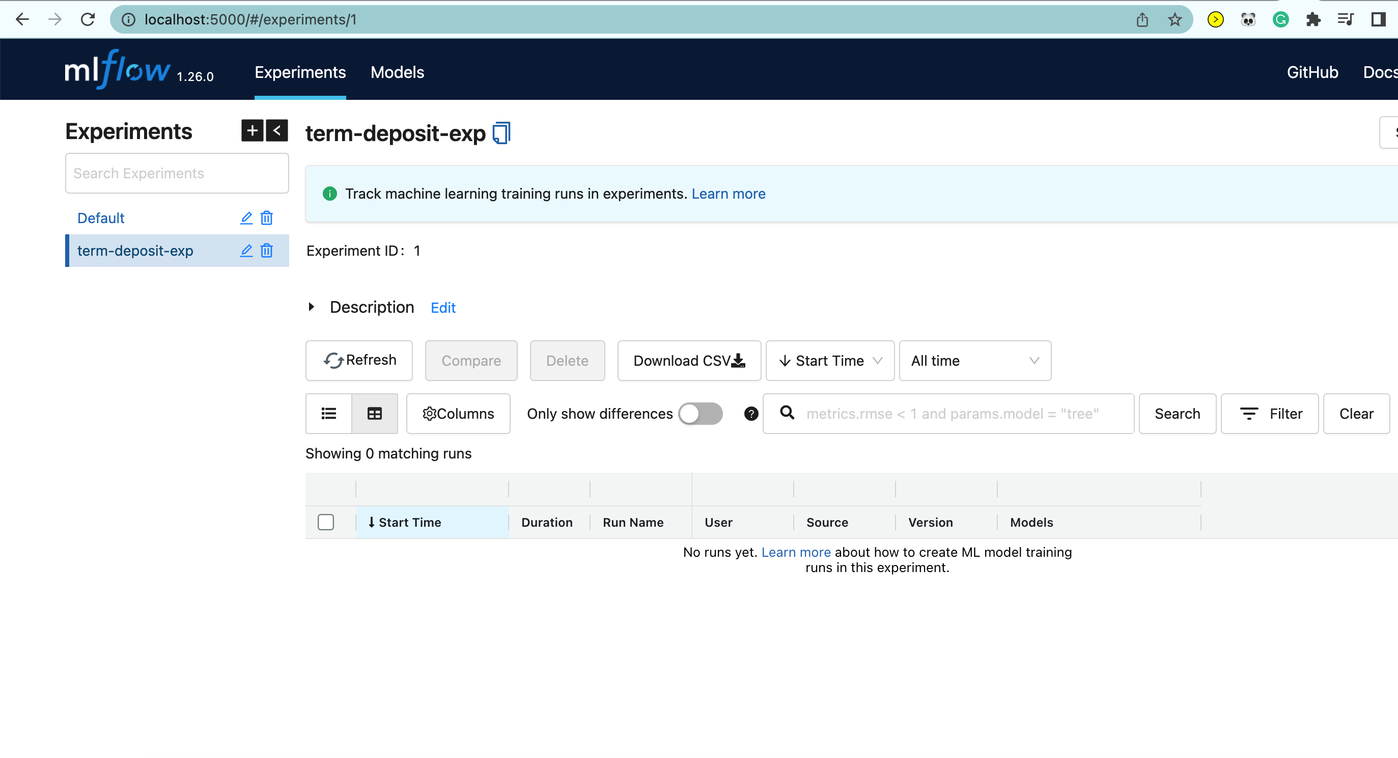
After running mlflow ui in the current working directory, you should have something like this:

We can populate the table once we tell mlflow to track any of our ML activities.
So let's get started. [Back to this Notebook]
# to make mlflow store your model files (artifacts) to a db, we have to define that
# we can work with sqlite

mlflow.set_tracking_uri("sqlite:///mlflow.db")
so now, you can go back to the terminal and run mlflow ui --backend-uri-sqlite:///mlflow.db. This will produce the same mlflow ui except that you can now open the Models tab (beside Experiments).
2. Refactor the codes
def load_data(train_path:str, test_path:str):
    train = pd.read_csv(train_path, sep=";")
    test = pd.read_csv(test_path, sep=";")

    return train, test


def preprocess_data(train_data, test_data):

    dv = DictVectorizer()

    trainX = train_data.drop(columns=["y"])
    trainy = train_data["y"]

    testX = test_data.drop(columns=["y"])
    testy = test_df["y"]

    trainy = trainy.replace({"no":0, "yes": 1})
    testy = testy.replace({"no":0, "yes": 1})

    trainX = dv.fit_transform(trainX.to_dict(orient="records")).toarray()

    testX = dv.fit_transform(testX.to_dict(orient="records")).toarray()

    return dv, trainX, trainy, testX, testy


def train_model(trainX, trainy, testX, testy):

    xgb = XGBClassifier()

    xgb.fit(trainX, trainy)

    pred = xgb.predict(testX)

    return xgb, pred


def evaluate(testy, pred):

    return (f1_score(testy, pred))
# save the model and dict vectorizer

def save_model(path:str, model, encoder):

    with open(path, "wb") as f_out:
        pickle.dump((model, encoder), f_out)

    return path
The four functions in the two cells above are a summary of all we've done previously. The last cell is for saving the model and encoder as a pickle file.
We will call all the functions in the next cell, but wrapped under mlflow.start_run().
3. Log the experiment
with mlflow.start_run(): # first start

    mlflow.set_tag("developer", "your_name") # tell mlflow to record your name.

    mlflow.log_param("train-data", "train.csv") # log the data path if you want
    mlflow.log_param("test-data", "test.csv")

    train, test = load_data("train.csv", "test.csv") # call the first function
    dv, trainX, trainy, testX, testy = preprocess_data(train, test) # call the second function

    xgb, pred = train_model(trainX, trainy, testX, testy) # call the third function

    # you can also log hyperparameters of the model.
    # for example: mlflow.log_params("max_leaves", "4")

    score = evaluate(testy, pred) # call the fourth function

    print(score)

    model_path = save_model("term-deposit.bin", xgb, dv) # save the model

    mlflow.log_metric("f1_score", score) # tell mlflow to record the model score

    # tell mlflow where to pick the model from and where to store it at:
    mlflow.log_artifact(local_path=model_path, artifact_path="xgb-model") # tell mlflow to store the model too.
There is also another way of logging the model to mlflow since we are using xgboost.
So instead of: mlflow.log_artifact(local_path="term-deposit.bin", artifact_path="xgb-model")
Do: mlflow.xgboost.log_model(xgb, artifact_path="xgb-model-version") as shown the cell below.
NOTE: The cell below is an alternative to the one above. You can run both to see the difference, but ensure you use different artifact paths
The latter is better because it stores more information about the model.
with mlflow.start_run(): # first start

    mlflow.set_tag("developer", "your_name") # tell mlflow to record your name.

    mlflow.log_param("train-data", "train.csv") # log the data path if you want
    mlflow.log_param("test-data", "test.csv")

    train, test = load_data("train.csv", "test.csv") # call the first function
    dv, trainX, trainy, testX, testy = preprocess_data(train, test) # call the second function

    xgb, pred = train_model(trainX, trainy, testX, testy) # call the third function

    # you can also log hyperparameters of the model.
    # for example: mlflow.log_params("max_leaves", "4")

    score = evaluate(testy, pred) # call the fourth function

    print(score)

    model_path = save_model("term-deposit.bin", xgb, dv)

    mlflow.log_metric("f1_score", score)

    # changes are from here:

    # pickle dump just the dict vectoriser
    with open("preprocessor.b", "wb") as f_out:
        pickle.dump(dv, f_out)

    # log the dict vectoriser
    mlflow.log_artifact("preprocessor.b", artifact_path="preprocessor")

    # log the model directly using .xgboost
    mlflow.xgboost.log_model(xgb, artifact_path="xgb-model-version")
After successfully running the cell above, you should now have mlflow.db file in your working directory. To view it from the ui, go back to your terminal and run this now:
mlflow ui --backend-store-uri sqlite:///mlflow.db
Remember to run this in your working directory, as you did previously and also ensure your environment is activated.
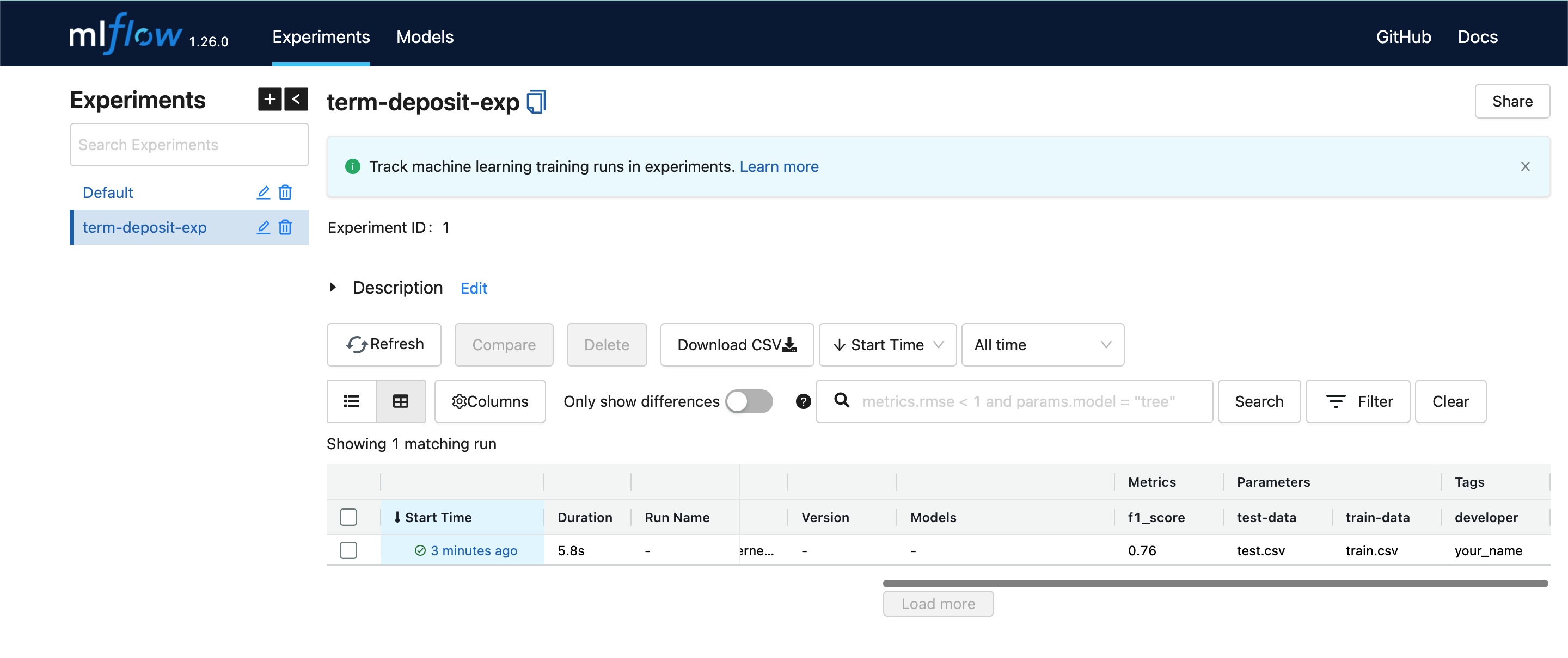
Your interface should be looking similar to mine below. Click on the time under the "Start Time" column, to see more details of the model and the artifacts.

Voila! We've come to the end of this note that introduces model experiementation with MLFlow.
THANKS FOR READING.